AI / TensorFlow Lite for Microcontrollers - 4. Hello World Training


TensorFlow Lite for Microcontrollers
Hello World Training
Hello World Training에서는 2.5 kB Model (generate a sine wave)을 실습해 볼 것이다.
데이터셋
1. 데이터 생성하기
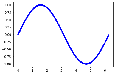
다음 셀의 코드는 일련의 랜덤 x값을 생성하고, 해당 사인값을 계산하여 그래프에 표시한다.
1
2
3
4
5
6
7
8
9
10
11
12
13
14
15
16
17
# Number of sample datapoints
SAMPLES = 1000

# Generate a uniformly distributed set of random numbers in the range from
# 0 to 2π, which covers a complete sine wave oscillation
x_values = np.random.uniform(
    low=0, high=2*math.pi, size=SAMPLES).astype(np.float32)

# Shuffle the values to guarantee they're not in order
np.random.shuffle(x_values)

# Calculate the corresponding sine values
y_values = np.sin(x_values).astype(np.float32)

# Plot our data. The 'b.' argument tells the library to print blue dots.
plt.plot(x_values, y_values, 'b.')
plt.show()
$[Fig.\,1]$
2. 노이즈 추가
사인함수에 의해 직접 생성되었기 때문에 이 데이터는 멋지고 부드러운 곡선이다.
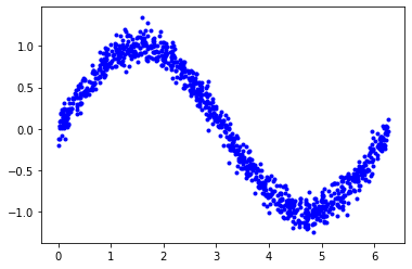
그러나 기계학습 모델은 지저분한 실제 데이터에서 기본적인 의미를 추출하는 데 능숙하다. 이를 입증하기 위해 데이터에 약간의 노이즈를 추가하여 보다 실제적인 것으로 추정할 수 있다.
다음 코드는 각 값에 약간의 무작위 노이즈를 추가한 다음 새 그래프를 그린다.
1
2
3
4
5
6
# Add a small random number to each y value
y_values += 0.1 * np.random.randn(*y_values.shape)

# Plot our data
plt.plot(x_values, y_values, 'b.')
plt.show()
$[Fig.\,2]$
3. 데이터 분할
이제 실제 데이터와 유사한 노이즈가 많은 데이터셋이 제공된다. 이것을 가지고 모델을 훈련시키는 데 사용할 수 있다.
훈련한 모델의 정확성을 평가하기 위해 예측값을 실제 데이터와 비교하여 예측값이 얼마나 잘 일치하는지 확인해야 한다. 이 평가는 훈련중(유효성 확인) 및 훈련후(테스트)에 실시된다. 두 경우 모두 모델을 훈련하는데 아직 사용되지 않은 새로운 데이터를 사용하는 것이 중요하다.
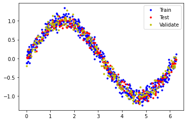
데이터는 다음과 같이 분할된다.
훈련: 60%
유효성 검사: 20%
테스트: 20%
이 분할 비율은 통상적으로 많이 사용된다.
다음 코드는 데이터를 분할한 다음 각 세트를 다른 색상으로 표시한다.
1
2
3
4
5
6
7
8
9
10
11
12
13
14
15
16
17
18
19
20
# We'll use 60% of our data for training and 20% for testing. The remaining 20%
# will be used for validation. Calculate the indices of each section.
TRAIN_SPLIT =  int(0.6 * SAMPLES)
TEST_SPLIT = int(0.2 * SAMPLES + TRAIN_SPLIT)

# Use np.split to chop our data into three parts.
# The second argument to np.split is an array of indices where the data will be
# split. We provide two indices, so the data will be divided into three chunks.
x_train, x_test, x_validate = np.split(x_values, [TRAIN_SPLIT, TEST_SPLIT])
y_train, y_test, y_validate = np.split(y_values, [TRAIN_SPLIT, TEST_SPLIT])

# Double check that our splits add up correctly
assert (x_train.size + x_validate.size + x_test.size) ==  SAMPLES

# Plot the data in each partition in different colors:
plt.plot(x_train, y_train, 'b.', label="Train")
plt.plot(x_test, y_test, 'r.', label="Test")
plt.plot(x_validate, y_validate, 'y.', label="Validate")
plt.legend()
plt.show()
$[Fig.\,3]$
훈련
0. 훈련 결과물
| Name | Format | Target Framework | Target Device |
|---|---|---|---|
model.pb | Keras SavedModel | TensorFlow | Large-Scale/Cloud/Servers |
model.tflite(2.5kB) | Integer Only Quantized TFLite Model | TensorFlow Lite | Mobile Devices |
model.cc | C Source File | TensorFlow Lite for Microcontrollers | Microcontrollers |
$[Table\,1]$
.pb: TensorFlow의 Protocol Buffer
.tflite: FlatBuffer의 TensorFlow Lite
mocdel.cc: C파일, const struct
1. 모델 설계
입력값(x)을 취하여 숫자 출력값(x의 사인)을 예측하는 간단한 뉴럴 네트워크 모델을 구축할 것이다. 이러한 유형의 문제를 회귀(regression)라고 한다. 이는 뉴런층을 사용하여 훈련 데이터의 기반이 되는 패턴을 학습하여 예측을 할 수 있도록 한다.
이를 위해 간단한 신경망을 만들텐데, 뉴런(neurons)과 레이어(layers)를 사용하여 훈련 데이터의 기본적인 패턴을 학습을 통해 예측을 수행한다.
우선, 두 개의 레이어를 정의한다. 첫 번째 층은 하나의 입력(x값)을 취해서 16개의 뉴런을 통과시킨다. 이 입력에 기초하여, 각각의 뉴런은 내부 상태(가중치weight 및 편향bias값)에 따라 어느 정도 활성화 될 것이다. 뉴런의 활성화 정도는 숫자로 표현된다.
첫 번째 층의 활성화 번호는 단일 뉴런인 두 번째 층에 대한 입력으로 공급된다. 이 입력에 자체 weight와 bias를 적용하고 활성화 정도 를 계산하여 y로 출력한다.
다음 코드는 TensorFlow의 딥러닝 네트워크 생성을 위한 상위 레벨 API인 Keras를 사용하는 모델을 정의한다. 네트워크가 정의되면 다음을 컴파일하여 교육 방법을 결정하는 매개변수를 지정한다.
1
2
3
4
5
6
7
8
9
10
11
12
# We'll use Keras to create a simple model architecture
model_1 = tf.keras.Sequential()

# First layer takes a scalar input and feeds it through 16 "neurons". The
# neurons decide whether to activate based on the 'relu' activation function.
model_1.add(keras.layers.Dense(16, activation='relu', input_shape=(1,)))

# Final layer is a single neuron, since we want to output a single value
model_1.add(keras.layers.Dense(1))

# Compile the model using the standard 'adam' optimizer and the mean squared error or 'mse' loss function for regression.
model_1.compile(optimizer='adam', loss='mse', metrics=['mae'])
2. 모델 훈련하기
모델을 정의한 후에는 데이터를 사용하여 훈련할 수 있다. 훈련은 x값을 뉴럴 네트워크로 전달, 네트워크의 출력이 예상 y값에서 얼마나 벗어나는지를 확인하고, 뉴런의 weight와 bias을 조정하여 다음에 출력이 더 정확할 수 있도록 하는 것을 포함한다.
훈련은 전체 데이터셋에서 이 프로세스를 여러 번 실행하며, 각 전체 실행 과정을 epoch라고 한다. 훈련중에 실행할 epoch의 수는 설정할 수 있는 매개변수이다.
각 epoch 동안 데이터는 여러 batches로 네트워크를 통해 실행된다. 각 batch마다 여러 개의 데이터가 네트워크로 전달되어 출력 값이 생성된다. 이러한 출력의 정확성은 총체적으로 측정되며, 그에 따라 네트워크의 weight와 bias가 batch당 한 번씩 조정된다. batch 크기는 설정할 수 있는 매개 변수이기도 하다.
다음 코드는 모델을 훈련하기 위해 훈련 데이터의 x 및 y 값을 사용한다. 각 batch에 64개의 데이터가 있는 500개의 epochs을 실행한다. 또한 검증을 위해 몇 가지 데이터도 전달한다. 훈련을 완료하는 데 시간이 걸릴 수 있다.
1
2
3
# Train the model on our training data while validating on our validation set
history_1 = model_1.fit(x_train, y_train, epochs=500, batch_size=64,
                        validation_data=(x_validate, y_validate))
1
2
3
4
5
6
7
8
9
10
11
12
13
14
15
16
17
18
19
20
21
22
23
Epoch 1/500
10/10 [==============================] - 1s 47ms/step - loss: 0.7289 - mae: 0.7120 - val_loss: 0.6401 - val_mae: 0.6504
Epoch 2/500
10/10 [==============================] - 0s 6ms/step - loss: 0.6329 - mae: 0.6488 - val_loss: 0.5587 - val_mae: 0.6031
Epoch 3/500
10/10 [==============================] - 0s 6ms/step - loss: 0.5201 - mae: 0.5735 - val_loss: 0.5014 - val_mae: 0.5763
Epoch 4/500
10/10 [==============================] - 0s 6ms/step - loss: 0.5057 - mae: 0.5760 - val_loss: 0.4632 - val_mae: 0.5615
Epoch 5/500
10/10 [==============================] - 0s 5ms/step - loss: 0.4502 - mae: 0.5459 - val_loss: 0.4386 - val_mae: 0.5536

...

Epoch 496/500
10/10 [==============================] - 0s 7ms/step - loss: 0.1754 - mae: 0.3581 - val_loss: 0.1848 - val_mae: 0.3695
Epoch 497/500
10/10 [==============================] - 0s 6ms/step - loss: 0.1729 - mae: 0.3563 - val_loss: 0.1847 - val_mae: 0.3687
Epoch 498/500
10/10 [==============================] - 0s 6ms/step - loss: 0.1727 - mae: 0.3584 - val_loss: 0.1847 - val_mae: 0.3688
Epoch 499/500
10/10 [==============================] - 0s 6ms/step - loss: 0.1713 - mae: 0.3522 - val_loss: 0.1847 - val_mae: 0.3685
Epoch 500/500
10/10 [==============================] - 0s 7ms/step - loss: 0.1634 - mae: 0.3428 - val_loss: 0.1846 - val_mae: 0.3680
3. Plot Matrics
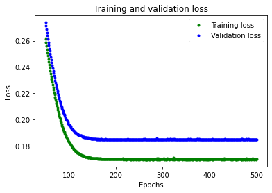
1) 손실(평균 제곱 오차)
훈련중 모델의 성능은 NAT의 훈련 데이터와 앞에서 설정한 검증 데이터 모두에 대해 지속적으로 측정된다. 훈련은 훈련 과정 동안 모델의 성능이 어떻게 변했는지 알려주는 데이터 로그를 생성한다.
다음 코드는 해당 데이터의 일부를 그래픽 형식으로 표시한다.
1
2
3
4
5
6
7
8
9
10
11
12
13
14
# Draw a graph of the loss, which is the distance between
# the predicted and actual values during training and validation.
train_loss = history_1.history['loss']
val_loss = history_1.history['val_loss']

epochs = range(1, len(train_loss) + 1)

plt.plot(epochs, train_loss, 'g.', label='Training loss')
plt.plot(epochs, val_loss, 'b', label='Validation loss')
plt.title('Training and validation loss')
plt.xlabel('Epochs')
plt.ylabel('Loss')
plt.legend()
plt.show()
$[Fig.\,4]$
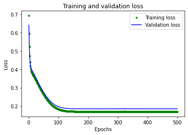
그래프는 각 epoch에 대한 손실(모델의 예측과 실제 데이터 간의 차이)을 보여준다. 손실을 계산하는 방법에는 여러 가지가 있으며, 여기서 사용한 방법은 평균 제곱 오차이다. 훈련과 검증 데이터에 대해 분명한 손실 값이 제시된다.
여기서 볼 수 있듯이, 손실의 양은 처음 25개 epoch에 걸쳐 급격히 감소하다가 평탄해진다. 이는 모델이 개선되고 더 정확한 예측을 만들어 내고 있다는 것을 의미한다.
모델이 더 이상 개선되지 않거나 훈련 손실이 검증 손실보다 적을 때 훈련을 중단하는 것이 목표이다. 이는 모델이 훈련 데이터를 너무 잘 예측하여 더 이상 새로운 데이터로 일반화하지 못한다는 것을 의미한다.
그래프의 평탄한 부분을 더 쉽게 읽을 수 있도록 처음 50개 epochs를 건너뛰겠다.
1
2
3
4
5
6
7
8
9
10
# Exclude the first few epochs so the graph is easier to read
SKIP = 50

plt.plot(epochs[SKIP:], train_loss[SKIP:], 'g.', label='Training loss')
plt.plot(epochs[SKIP:], val_loss[SKIP:], 'b.', label='Validation loss')
plt.title('Training and validation loss')
plt.xlabel('Epochs')
plt.ylabel('Loss')
plt.legend()
plt.show()
$[Fig.\,5]$
그림에서 손실은 200여개의 epochs까지 계속 감소한다는 것을 알 수 있으며, 이때 손실은 대부분 안정적이다. 즉, 200개 epochs를 넘어서는 네트워크를 훈련할 필요가 없다.
그러나 가장 낮은 손실값은 여전히 0.155 정도이다. 이는 네트워크의 예측이 평균 15%까지 어긋난다는 것을 의미한다. 또한 검증 손실 값이 크게 증가하며 때로는 훨씬 더 높다.
2) 평균 절대 오차
모델의 성능에 대한 더 많은 정보를 얻기 위해 데이터를 추가로 플롯팅할 수 있다. 이번에는 평균 절대 오차를 표시하겠다. 이는 네트워크의 예측이 실제 수치와 얼마나 멀리 떨어져 있는지를 측정하는 또 다른 방법이다.
1
2
3
4
5
6
7
8
9
10
11
12
13
14
plt.clf()

# Draw a graph of mean absolute error, which is another way of
# measuring the amount of error in the prediction.
train_mae = history_1.history['mae']
val_mae = history_1.history['val_mae']

plt.plot(epochs[SKIP:], train_mae[SKIP:], 'g.', label='Training MAE')
plt.plot(epochs[SKIP:], val_mae[SKIP:], 'b.', label='Validation MAE')
plt.title('Training and validation mean absolute error')
plt.xlabel('Epochs')
plt.ylabel('MAE')
plt.legend()
plt.show()
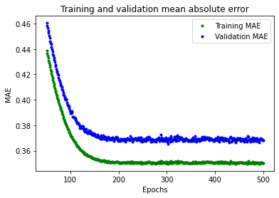
$[Fig.\,6]$
이 평균 절대 오차 그래프는 다른 타입이다. 훈련 데이터가 검증 데이터보다 일관되게 오류가 적다는 것을 알 수 있다. 즉, 네트워크가 overfit 되었거나 훈련 데이터를 너무 엄격하게 학습하여 새 데이터에 대한 효과적인 예측을 할 수 없다.
또한 평균 절대 오차 값은 잘해봐야 0.305로 상당히 높으며, 이는 모델의 예측 중 일부가 최소 30% 이상 차이가 난다는 것을 의미한다. 30% 오차는 사인파 함수를 정확하게 모델링하는 것과는 거리가 멀다는 것을 의미한다.
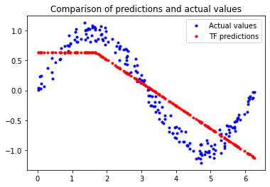
3) 실제 출력 vs 예측 출력
어떤 일이 일어나고 있는지 좀 더 자세히 알아보기 위해 앞서 정리해 둔 테스트 데이터셋과 예측 결과를 확인해 보겠다.
1
2
3
4
5
6
7
8
9
10
11
12
13
# Calculate and print the loss on our test dataset
test_loss, test_mae = model_1.evaluate(x_test, y_test)

# Make predictions based on our test dataset
y_test_pred = model_1.predict(x_test)

# Graph the predictions against the actual values
plt.clf()
plt.title('Comparison of predictions and actual values')
plt.plot(x_test, y_test, 'b.', label='Actual values')
plt.plot(x_test, y_test_pred, 'r.', label='TF predictions')
plt.legend()
plt.show()
$[Fig.\,7]$
1
7/7 [==============================] - 0s 2ms/step - loss: 0.1627 - mae: 0.34
이 그래프는 네트워크가 매우 제한된 방법으로 사인 함수를 근사하는 방법을 학습했음을 분명히 보여준다.
이 fit의 硬直性(경직성)은 모델이 사인파 기능의 전체 복잡성을 학습하기에 충분한 용량이 없다는 것을 시사한다. 따라서 매우 단순화된 방법으로만 근사치를 계산할 수 있다. 모델을 더 크게 만들어서 성능을 개선할 수 있을 것이다.
더 큰 모델 훈련
1. 모델 변경
모델을 더 크게 만들기 위해 뉴런층을 추가해 보겠다. 다음 코드는 이전과 같은 방식으로 모델을 재정의하지만 첫번째 층에는 16개의 뉴런이 있고 중간에 16개의 뉴런이 추가되어있다.
1
2
3
4
5
6
7
8
9
10
11
12
13
14
model = tf.keras.Sequential()

# First layer takes a scalar input and feeds it through 16 "neurons". The
# neurons decide whether to activate based on the 'relu' activation function.
model.add(keras.layers.Dense(16, activation='relu', input_shape=(1,)))

# The new second and third layer will help the network learn more complex representations
model.add(keras.layers.Dense(16, activation='relu'))

# Final layer is a single neuron, since we want to output a single value
model.add(keras.layers.Dense(1))

# Compile the model using the standard 'adam' optimizer and the mean squared error or 'mse' loss function for regression.
model.compile(optimizer='adam', loss="mse", metrics=["mae"])
2. 모델 다시 훈련
이제 새 모델을 훈련하여 저장할 것이다.
1
2
3
4
5
6
# Train the model
history = model.fit(x_train, y_train, epochs=500, batch_size=64,
                    validation_data=(x_validate, y_validate))

# Save the model to disk
model.save(MODEL_TF)
1
2
3
4
5
6
7
8
9
10
11
12
13
14
15
16
17
18
19
20
21
22
23
Epoch 1/500
10/10 [==============================] - 1s 20ms/step - loss: 0.4355 - mae: 0.5542 - val_loss: 0.4315 - val_mae: 0.5685
Epoch 2/500
10/10 [==============================] - 0s 5ms/step - loss: 0.4183 - mae: 0.5548 - val_loss: 0.4157 - val_mae: 0.5581
Epoch 3/500
10/10 [==============================] - 0s 6ms/step - loss: 0.3871 - mae: 0.5322 - val_loss: 0.3988 - val_mae: 0.5444
Epoch 4/500
10/10 [==============================] - 0s 5ms/step - loss: 0.3954 - mae: 0.5348 - val_loss: 0.3834 - val_mae: 0.5350
Epoch 5/500
10/10 [==============================] - 0s 5ms/step - loss: 0.3670 - mae: 0.5163 - val_loss: 0.3684 - val_mae: 0.5257

...

Epoch 496/500
10/10 [==============================] - 0s 6ms/step - loss: 0.0118 - mae: 0.0861 - val_loss: 0.0114 - val_mae: 0.0863
Epoch 497/500
10/10 [==============================] - 0s 6ms/step - loss: 0.0107 - mae: 0.0818 - val_loss: 0.0115 - val_mae: 0.0864
Epoch 498/500
10/10 [==============================] - 0s 7ms/step - loss: 0.0123 - mae: 0.0894 - val_loss: 0.0114 - val_mae: 0.0862
Epoch 499/500
10/10 [==============================] - 0s 6ms/step - loss: 0.0126 - mae: 0.0895 - val_loss: 0.0113 - val_mae: 0.0857
Epoch 500/500
10/10 [==============================] - 0s 6ms/step - loss: 0.0121 - mae: 0.0882 - val_loss: 0.0115 - val_mae: 0.0865
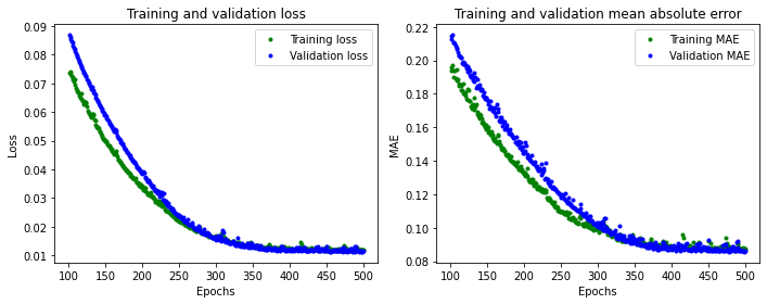
3. 새로운 Plot Matrics
각 훈련 epoch마다 모델은 손실과 훈련 및 검증을 위한 평균 절대 오류를 출력한다. 위의 출력에서 이 내용을 읽을 수 있다.
1
2
Epoch 500/500
10/10 [==============================] - 0s 10ms/step - loss: 0.0121 - mae: 0.0882 - val_loss: 0.0115 - val_mae: 0.0865
검증 손실은 0.15에서 0.01로, 검증 MAE는 0.33에서 0.08로 크게 개선되었다.
다음 코드는 원래 모델을 평가하는 데 사용한 그래프와 동일한 그래프를 출력하지만 새로운 모델 history를 보여준다.
1
2
3
4
5
6
7
8
9
10
11
12
13
14
15
16
17
18
19
20
21
22
23
24
25
26
27
28
29
30
31
32
33
34
35
# Draw a graph of the loss, which is the distance between
# the predicted and actual values during training and validation.
train_loss = history.history['loss']
val_loss = history.history['val_loss']

epochs = range(1, len(train_loss) + 1)

# Exclude the first few epochs so the graph is easier to read
SKIP = 100

plt.figure(figsize=(10, 4))
plt.subplot(1, 2, 1)

plt.plot(epochs[SKIP:], train_loss[SKIP:], 'g.', label='Training loss')
plt.plot(epochs[SKIP:], val_loss[SKIP:], 'b.', label='Validation loss')
plt.title('Training and validation loss')
plt.xlabel('Epochs')
plt.ylabel('Loss')
plt.legend()

plt.subplot(1, 2, 2)

# Draw a graph of mean absolute error, which is another way of
# measuring the amount of error in the prediction.
train_mae = history.history['mae']
val_mae = history.history['val_mae']

plt.plot(epochs[SKIP:], train_mae[SKIP:], 'g.', label='Training MAE')
plt.plot(epochs[SKIP:], val_mae[SKIP:], 'b.', label='Validation MAE')
plt.title('Training and validation mean absolute error')
plt.xlabel('Epochs')
plt.ylabel('MAE')
plt.legend()

plt.tight_layout()
$[Fig.\,8]$
좋은 결과가 나왔다. 이 그래프에서 몇 가지 흥미로운 점을 볼 수 있다.
- 전체적인 손실과
MAE는 이전 네트워크보다 훨씬 더 우수하다. - 훈련보다 검증에 더 적합한 Matrics, 즉 네트워크가 과적합하지 않음을 의미한다.
훈련을 위한 메트릭보다 검증 Matrics이 더 나은 이유는, 검증 Matrics가 각 epoch 마지막에 계산되는 반면, 훈련 Matrics은 epoch 전체에서 계산되므로 약간 더 오랜 시간 훈련받은 모델에서 검증이 수행되기 때문이다.
이 모든 것은 이 네트워크가 잘 작동하는 것 같다는 것을 의미한다. 먼저 예측 결과를 앞서 정리해 둔 테스트 데이터셋과 비교하여 확인해 보겠다.
1
2
3
4
5
6
7
8
9
10
11
12
13
# Calculate and print the loss on our test dataset
test_loss, test_mae = model.evaluate(x_test, y_test)

# Make predictions based on our test dataset
y_test_pred = model.predict(x_test)

# Graph the predictions against the actual values
plt.clf()
plt.title('Comparison of predictions and actual values')
plt.plot(x_test, y_test, 'b.', label='Actual values')
plt.plot(x_test, y_test_pred, 'r.', label='TF predicted')
plt.legend()
plt.show()
1
7/7 [==============================] - 0s 2ms/step - loss: 0.0102 - mae: 0.081
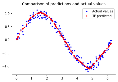
$[Fig.\,9]$
훨씬 나아졌다. 우리가 출력한 평가 지표는 모델의 손실이 적고 테스트 데이터에 MAE가 있다는 것을 보여주며, 예측은 우리의 데이터에 시각적으로 잘 들어맞는다.
모델은 완벽하지 않다. 예측은 부드러운 사인 곡선을 형성하지 않는다. 예를 들어, x가 4.2와 5.2사이일 때 선은 거의 직선이다. 한 단계 더 나아가려면 모델의 용량을 더 늘릴 수 있다. overfit을 방지하기 위해 몇 가지 기술을 사용할 수도 있다.
하지만 기계학습의 중요한 부분은 언제 멈출지 아는 것이다. 이 모델은 일부 LED가 안정된 패턴으로 깜박이게 하는 사용 사례에 적합하다.
TensorFlow Lite 모델로 변환
1. 양자화 관계없이 모델 생성
이제 어느 정도 정확한 모델을 가지고 있다. TensorFlow Lite Converter를 사용하여 메모리 제약이 있는 장치에 사용할 수 있도록 모델을 특수하고 공간 효율적인 형식으로 변환한다.
이 모델은 마이크로 컨트롤러에 구축될 예정이므로 가능한 한 작게 제작해야한다. 모델의 크기를 줄이는 한 가지 기술은 양자화라고한다. 이는 모델 weight 정밀도를 떨어뜨리고, 활성화(각 레이어의 출력)도 감소시켜 종종 정확도에 큰 영향을 미치지 않고 메모리를 절약한다. 양자화된 모델도 더 빠르게 실행된다. 필요한 계산이 더 간단하기 때문이다.
다음 코드에서는 모델을 두번 변환한다. 하나는 양자화한 모델, 다른 하나는 하지 않은 모델.
1
2
3
4
5
6
7
8
9
10
11
12
13
14
15
16
17
18
19
20
21
22
23
# Convert the model to the TensorFlow Lite format without quantization
converter = tf.lite.TFLiteConverter.from_saved_model(MODEL_TF)
model_no_quant_tflite = converter.convert()

# Save the model to disk
open(MODEL_NO_QUANT_TFLITE, "wb").write(model_no_quant_tflite)

# Convert the model to the TensorFlow Lite format with quantization
def representative_dataset():
  for i in range(500):
    yield([x_train[i].reshape(1, 1)])
# Set the optimization flag.
converter.optimizations = [tf.lite.Optimize.DEFAULT]
# Enforce integer only quantization
converter.target_spec.supported_ops = [tf.lite.OpsSet.TFLITE_BUILTINS_INT8]
converter.inference_input_type = tf.int8
converter.inference_output_type = tf.int8
# Provide a representative dataset to ensure we quantize correctly.
converter.representative_dataset = representative_dataset
model_tflite = converter.convert()

# Save the model to disk
open(MODEL_TFLITE, "wb").write(model_tflite)
1
2488
2. 모델 성능 비교
변환 및 양자화 후에도 이러한 모델이 정확하다는 것을 입증하기 위해 테스트 데이터셋에서 예측 및 손실을 비교할 것이다.
Helper functions
TFLite 모델에 대한 예측을 정의하고 손실 함수를 평가한다. (TF 모델에는 이미 포함되어 있지만 TFLite 모델에는 포함되어 있지 않다.)
1
2
3
4
5
6
7
8
9
10
11
12
13
14
15
16
17
18
19
20
21
22
23
24
25
26
27
28
29
30
31
32
33
34
35
36
37
38
39
40
def predict_tflite(tflite_model, x_test):
    # Prepare the test data
    x_test_ = x_test.copy()
    x_test_ = x_test_.reshape((x_test.size, 1))
    x_test_ = x_test_.astype(np.float32)

    # Initialize the TFLite interpreter
    interpreter = tf.lite.Interpreter(model_content=tflite_model)
    interpreter.allocate_tensors()

    input_details = interpreter.get_input_details()[0]
    output_details = interpreter.get_output_details()[0]

    # If required, quantize the input layer (from float to integer)
    input_scale, input_zero_point = input_details["quantization"]
    if (input_scale, input_zero_point) != (0.0, 0):
        x_test_ = x_test_ / input_scale + input_zero_point
        x_test_ = x_test_.astype(input_details["dtype"])

    # Invoke the interpreter
    y_pred = np.empty(x_test_.size, dtype=output_details["dtype"])
    for i in range(len(x_test_)):
        interpreter.set_tensor(input_details["index"], [x_test_[i]])
        interpreter.invoke()
        y_pred[i] = interpreter.get_tensor(output_details["index"])[0]

    # If required, dequantized the output layer (from integer to float)
    output_scale, output_zero_point = output_details["quantization"]
    if (output_scale, output_zero_point) != (0.0, 0):
        y_pred = y_pred.astype(np.float32)
        y_pred = (y_pred - output_zero_point) * output_scale

    return y_pred

def evaluate_tflite(tflite_model, x_test, y_true):
    global model
    y_pred = predict_tflite(tflite_model, x_test)
    loss_function = tf.keras.losses.get(model.loss)
    loss = loss_function(y_true, y_pred).numpy()
    return loss
1) Predictions
1
2
3
4
# Calculate predictions
y_test_pred_tf = model.predict(x_test)
y_test_pred_no_quant_tflite = predict_tflite(model_no_quant_tflite, x_test)
y_test_pred_tflite = predict_tflite(model_tflite, x_test)
1
2
3
4
5
6
7
8
9
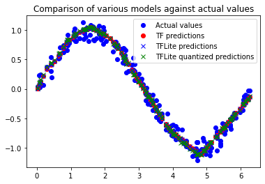
# Compare predictions
plt.clf()
plt.title('Comparison of various models against actual values')
plt.plot(x_test, y_test, 'bo', label='Actual values')
plt.plot(x_test, y_test_pred_tf, 'ro', label='TF predictions')
plt.plot(x_test, y_test_pred_no_quant_tflite, 'bx', label='TFLite predictions')
plt.plot(x_test, y_test_pred_tflite, 'gx', label='TFLite quantized predictions')
plt.legend()
plt.show()
$[Fig.\,10]$
2) Loss (MSE/Mean Squared Error)
1
2
3
4
# Calculate loss
loss_tf, _ = model.evaluate(x_test, y_test, verbose=0)
loss_no_quant_tflite = evaluate_tflite(model_no_quant_tflite, x_test, y_test)
loss_tflite = evaluate_tflite(model_tflite, x_test, y_test)
1
2
3
4
5
6
7
# Compare loss
df = pd.DataFrame.from_records(
    [["TensorFlow", loss_tf],
     ["TensorFlow Lite", loss_no_quant_tflite],
     ["TensorFlow Lite Quantized", loss_tflite]],
     columns = ["Model", "Loss/MSE"], index="Model").round(4)
df
| Model | Loss/MSE |
|---|---|
| TensorFlow | 0.0102 |
| TensorFlow Lite | 0.0102 |
| TensorFlow Lite Quantized | 0.0108 |
$[Table\,2]$
3) Size
1
2
3
4
# Calculate size
size_tf = os.path.getsize(MODEL_TF)
size_no_quant_tflite = os.path.getsize(MODEL_NO_QUANT_TFLITE)
size_tflite = os.path.getsize(MODEL_TFLITE)
1
2
3
4
5
6
# Compare size
pd.DataFrame.from_records(
    [["TensorFlow", f"{size_tf} bytes", ""],
     ["TensorFlow Lite", f"{size_no_quant_tflite} bytes ", f"(reduced by {size_tf - size_no_quant_tflite} bytes)"],
     ["TensorFlow Lite Quantized", f"{size_tflite} bytes", f"(reduced by {size_no_quant_tflite - size_tflite} bytes)"]],
     columns = ["Model", "Size", ""], index="Model")
| Model | Size |
|---|---|
| TensorFlow | 4096 bytes |
| TensorFlow Lite | 2788 bytes (reduced by 1308 bytes) |
| TensorFlow Lite Quantized | 2488 bytes (reduced by 300 bytes) |
$[Table\,3]$
요약
Predictions($[Fig.\,10]$)과 Loss($[Table\,2]$)을 통해 원래의 TF 모델, TFLite 모델 및 양자화된 TFLite 모델은 Size($[Table\,3]$)가 다르지만 구별할 수 없을 정도로 가깝다는 것을 알 수 있다. 이는 양자화된 (최소) 모델을 사용할 준비가 되었음을 의미한다.
참고: 양자화된 (integer) TFLite 모델은 원래 (float) TFLite 모델보다 300바이트 작다. 이는 모델이 이미 너무 작아서 양자화 효과가 거의 없기 때문이다. weight가 더 많이 나가는 복잡한 모델은 크기를 최대 4배까지 줄일 수 있다.
TensorFlow Lite for Microcontrollers 모델로 변환
TensorFlow Lite 양자화 모델을 TensorFlow Lite for Microcontrollers에 의해 로드될 수 있는 C 소스 파일로 변환한다.
1
2
3
4
5
6
7
# Install xxd if it is not available
!apt-get update && apt-get -qq install xxd
# Convert to a C source file, i.e, a TensorFlow Lite for Microcontrollers model
!xxd -i {MODEL_TFLITE} > {MODEL_TFLITE_MICRO}
# Update variable names
REPLACE_TEXT = MODEL_TFLITE.replace('/', '_').replace('.', '_')
!sed -i 's/'{REPLACE_TEXT}'/g_model/g' {MODEL_TFLITE_MICRO}
1
2
3
4
5
6
7
8
9
10
11
12
Ign:1 https://developer.download.nvidia.com/compute/cuda/repos/ubuntu1804/x86_64  InRelease
Hit:2 https://cloud.r-project.org/bin/linux/ubuntu bionic-cran40/ InRelease
Ign:3 https://developer.download.nvidia.com/compute/machine-learning/repos/ubuntu1804/x86_64  InRelease
Hit:4 http://ppa.launchpad.net/c2d4u.team/c2d4u4.0+/ubuntu bionic InRelease
Hit:5 http://archive.ubuntu.com/ubuntu bionic InRelease
Hit:6 http://security.ubuntu.com/ubuntu bionic-security InRelease
Hit:7 https://developer.download.nvidia.com/compute/cuda/repos/ubuntu1804/x86_64  Release
Hit:8 https://developer.download.nvidia.com/compute/machine-learning/repos/ubuntu1804/x86_64  Release
Hit:9 http://archive.ubuntu.com/ubuntu bionic-updates InRelease
Hit:10 http://ppa.launchpad.net/graphics-drivers/ppa/ubuntu bionic InRelease
Hit:11 http://archive.ubuntu.com/ubuntu bionic-backports InRelease
Reading package lists... Done